Physics, acceleration and FIRE(^2)

Financial Independence / Early Retirement is about reaching a state, in which you get enough passive income to live. Let’s say you get $Y$ EUR each month. The overall money you get over time is $ M = Y * t $, where $t$ is time. This resembles a physics equation for movement with constant speed (i.e. no acceleration). Let’s explore this similarity and try to add acceleration to FIRE and get FIRE$^2$ (FIRE squared, I just made this name up).

Physics prelude

If an object moves with a constant speed $V$ in one dimensional space, then its position can be obtained by $x = V t + x_0$, where $t$ is time and $x_0$ is the initial position.

The case above assumes no acceleration (the speed is constant). If we have constant acceleration the equation becomes $x = \frac{a t^2}{2} + V t + x_0$.

Back to FIRE

In physics the object moves by $V$ for each unit of time. In FIRE one gets $Y$ EUR each month (i.e. unit of time). Basically, if we denote cumulative number of money obtained through FIRE as $C$, the equation is similar to the equation above:

$C = Y t$

Now let’s try to add acceleration here. The equation becomes:

$C = \frac{a t^2}{2} + Y t$ $Y = a t + \text{<initial value>}$

What does this mean? The first month we get $Y$. The second month we get already $Y + a$. The third - $Y + 2a$ and so on. In other words, the amount we get from FIRE each month (our speed) should grow by $a$ each month.

Let’s check whether equation above works as we expect. At $ t = 1 $ the value is $ C = \frac{a}{2} + Y $, but we expect only $ Y $. This is likely, because the speed in physics grows continuously, while here in FIRE the process is discrete. E.g. for $ t = 0.5 $, the formula above gives

$Y = 0.5 a + \text{<initial value>}$

Thus, let’s try to build our own equation then:

At time $ t = 0 $, we have 0 EUR overall and our monthly income is $ Y $.
$ t = 1 $, we get $ Y $, overall we have $ Y $ and our monthly income becomes $ Y + a $
$ t = 2 $, we get $ Y + a $, overall $ 2Y + a $, income $ Y + 2a $
$ t = 3 $, we get $ Y + 2a $, overall $ 3Y + 3a $, income $ Y + 3a $
$ t = 4 $, we get $ Y + 3a $, overall $ 4Y + 6a $, income $ Y + 4a $

As we can see the equation is

$C = t Y + \text{<something>} \cdot a$

At first we add no $ a $, then $ a $, then $ 2a $ and so on. Thus, this is just a sum of arithmetic progression. The formula for the general case is

$S = (x_1 + x_n) \frac{n}{2}$

(i.e. sum of the first $ x_1 $ and last $ x_n $ elements multiplied by quantity $ n $ and divided by two). In our case it is

$(0 + t-1) \frac{t}{2} = (t-1)\frac{t}{2}$

Our final formula becomes

$C = t Y + (t-1)\frac{t}{2} a$

Under $ t = 4 $, we get $ 4 Y + 3 \cdot \frac{4}{2} a = 4 Y + 6 a $. Thus, it matches our manual calculations above.

Even further back

Now I am curious to see how much money one needs to build such FIRE with acceleration (FIRE$^2$). In other words, what kind of safe withdrawal rate one needs for this (could be denotes as SWR$^2$).

Let’s say that we want our acceleration to be $ A $ and we start with 0 speed at first. After the first month we get $ A $ units of money. Under 4% SWR, we would need $ 25 \cdot 12 \cdot A $ EUR overall. After the second month we get $ 2A $ EUR. In the normal FIRE we would need $ 25 \cdot 12 \cdot 2 \cdot A $ EUR overall to achieve such withdrawal.

Ok, this approach does not bring us far. Instead let’s say that in the first month we get $ A_1 $ EUR and in the second month we want to get $ A_2 = A_1 + 1 $ EUR. This means that after $ A_1 $ our stash should grow such that it starts producing 1 EUR more. Under 4% SWR one needs $ 25 \cdot 12 \cdot 1 = 300 $ EUR to get 1 EUR per month. Thus, $ A_1 $ should be 300 EUR. Now we can try to extend this further. We want $ A_2 = A_1 + A $ EUR. Thus, $ A_1 $ should be $ 300A $.

Let’s consider an example. Our monthly FIRE target is $ 300A $ EUR. We have $ 25 \cdot 12 \cdot 300 \cdot A = 300^2 A $ EUR overall. After the first month we get

$300^2 A \cdot \frac{0.04}{12} = 300 A$

We reinvest them. Now our stash becomes $ 300^2 A + 300 A $ EUR. In the second month, we get

$(300^2 A + 300 A) \frac{0.04}{12} = 301 A$ .

Oops, we wanted $ 600 A $. So it feels like the compound interest works differently from the physics motion equation. Let’s say our principal is $ P $ EUR and it grows by 4% each year, then after $ n $ years we will have $ P \cdot 1.04 ^ n $. If we don’t spend anything, our monthly FIRE income after $ n $ years will be $ P \cdot 1.04 ^ n \frac{0.04}{12} $. In other words, in contrast to the motion equation, here the time $ n $ is in the power. Previously, it was just square multiplied. This is why our analogy breaks.

However, we know that $ Y = a t $. We can plug income from the above as $ Y $ here and see the acceleration (for simplicity we switch units to years here):

$Y = a n = P \cdot 1.04 ^ n \frac{0.04}{12}$ $a = \frac{ P \cdot 1.04 ^ n \frac{0.04}{12} }{n}$

In other words the acceleration is not constant, it grows as well. In some sense, the real 4% is even better than the constant acceleration case above. If we want $ Y $ to be $ 2A $, we need $ 2 A \cdot 12 \cdot 25 $ EUR stash. Let’s say our initial stash supports $ Y = A $, i.e. it is $ 12 \cdot 25 \cdot A $. We know that in $ n $ years it will be $ 12 \cdot 25 \cdot A \cdot 1.04 ^ n $. Thus, let’s find $ n $, such that $ Y = 2 A $, i.e. the stash of $ 2 * A * 12 * 25 $ EUR. This is just $ 1.04 ^ n = 2 $, i.e. $ n = 17.673 $ (wolfram alpha). That’s a long time, but when we want $ Y = 3 A $, $ n $ becomes 28.011. I.e. the jump from $ Y = 2 A $ to $ Y = 3 A $ takes us ~10 years, while the jump from $ A $ to $ 2 A $ takes 17 years. For $ 1000 A $, $ n $ is 176.125, while for $ 1001 A $, it is 176.151, i.e. one needs only ~10 days to go from $ Y = 1000 A $ to $ 1001 A $, because the acceleration of compounding is not constant.

We can visualize this well with a plot. Let’s draw $ Y $ for both cases (linear and compounding):

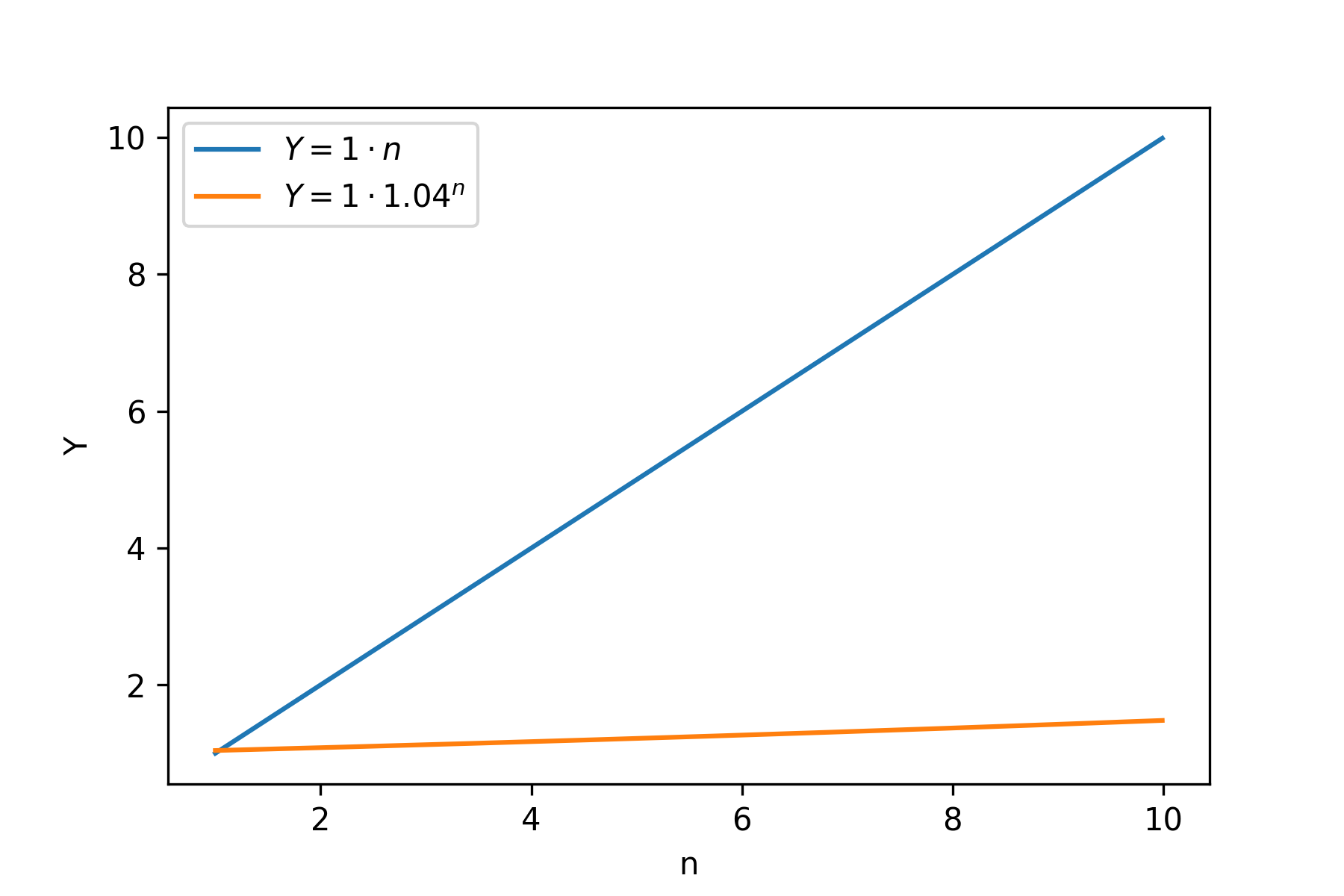
A plot showing how monthly FIRE income depends on time assuming linear and compounding growth.
Linear is much higher.

As we can see, linear is doing much better job at first. There is not much money to work in the compounding case yet. However, if we look further right:

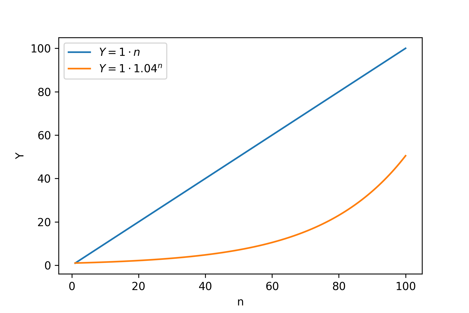
A plot showing how monthly FIRE income depends on time assuming linear and compounding growth.
This time we look from 1 to 100 on x axis and compounding almost reaches linear.

Compounding starts to reach linear. Even further right:

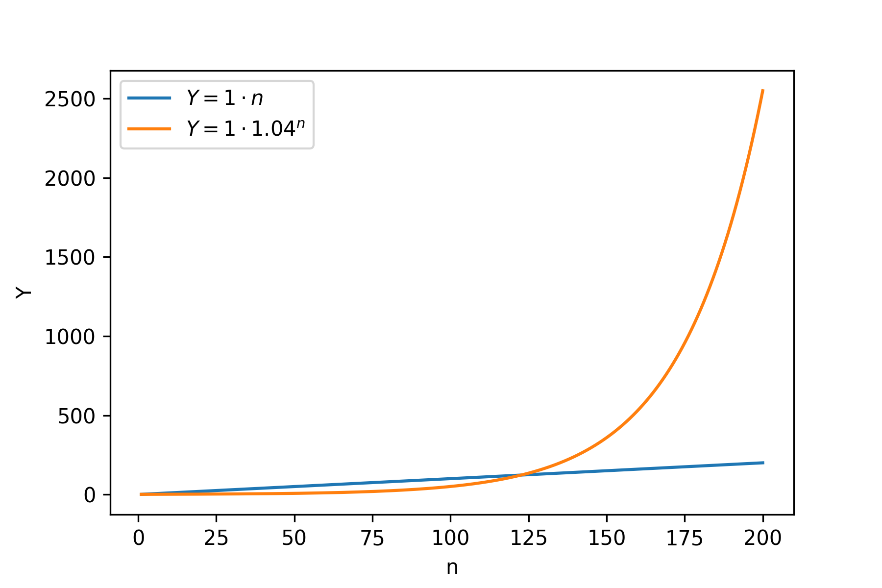
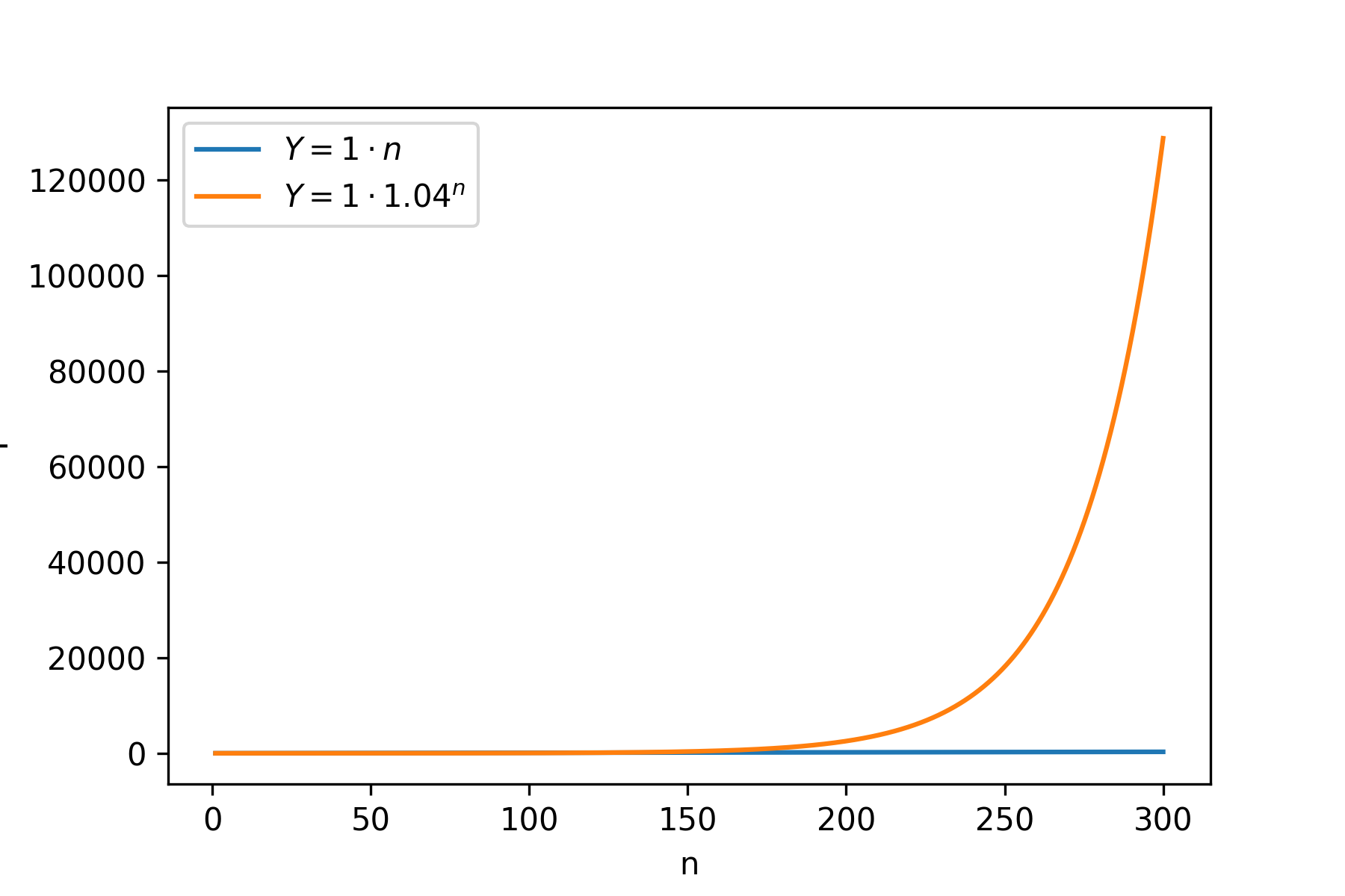
A plot showing how monthly FIRE income depends on time assuming linear and compounding growth.
This time we look from 1 to 200 on x axis and compounding sky-rockets.

And kaboom! Compounding case just skyrockets. Further to the right, it looks like linear is just flat:

A plot showing how monthly FIRE income depends on time assuming linear and compounding growth.
This time we look from 1 to 300 on x axis and linear looks completely flat.

Conclusions

Looking back, the fact that acceleration is not constant feels now obvious. Basically, when one has more money, compounding growth has more effect, because each euro works separately. While in the physics motion equation, the speed is just time multiplied by acceleration.

Thus, building such FIRE scheme when one each months gets $ A $ more money is not possible with the compounding growth. The compounding growth grows faster than that scheme (it just starts slow).

It is a bit sad that my attempt to define FIRE$^2$ and SWR$^2$ didn’t work out, because the real thing is in some sense cooler.

Possible follow-up

This didn’t workout, because the time goes into power. However, there is a way (logarithm) to move from exponent to linear. Thus, I could theoretically consider logarithm of the monthly income and try to do exactly the same.